NN-Z2H Lesson 6: Building makemore part 5 - Building a WaveNet

This is not orginal content!

This is my study notes / codes along with Andrej Karpathy’s “Neural Networks: Zero to Hero” series.

Codes are executed in Colab, this calculation capacity exceeds my computer’s ability.

1 intro

We are going to take the 2-layer MLP in the part 3 of makemore and complexify it by:

• extending the block size: from 3 to 8 characters;
• making it deeper rather than 1 hidden layer.

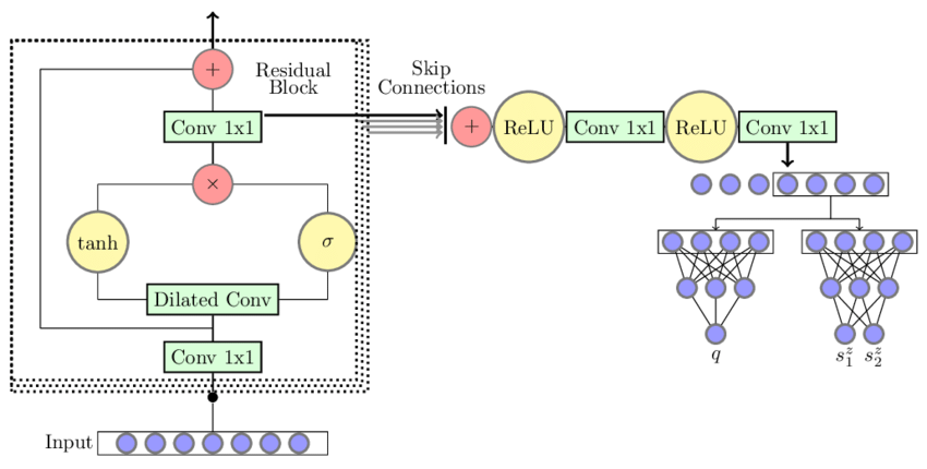
then end of with a Convoluntional Neural Network architecture similar to WaveNet (2016) by Google DeepMind.

WaveNet model architecture, source

starter code walk through

import libraries

import torch
import torch.nn.functional as F
import pandas as pd
import matplotlib.pyplot as plt
%matplotlib inline

reading data

import pandas as pd

url = "https://raw.githubusercontent.com/karpathy/makemore/refs/heads/master/names.txt"
words = pd.read_csv(url, header=None).iloc[:, 0].tolist()
words[:8]

# >>> ['emma', 'olivia', 'ava', 'isabella', 'sophia', 'charlotte', 'mia', 'amelia']

building vocab

# build the vocabulary of characters and mapping to/from integer
chars = sorted(list(set(''.join(words))))
stoi = {s:i+1 for i, s in enumerate(chars)}
stoi['.'] = 0
itos = {i: s for s, i in stoi.items()}
vocab_size = len(itos)
print(itos)
print(vocab_size)

# itos: {1: 'a', 2: 'b', 3: 'c', 4: 'd', 5: 'e', 6: 'f', 7: 'g', 8: 'h', 9: 'i', 10: 'j', 
# 11: 'k', 12: 'l', 13: 'm', 14: 'n', 15: 'o', 16: 'p', 17: 'q', 18: 'r', 19: 's', 20: 't', 
# 21: 'u', 22: 'v', 23: 'w', 24: 'x', 25: 'y', 26: 'z', 0: '.'}
# vocab_size: 27

initializing randomization

import random
random.seed(42)
random.shuffle(words)

create train/dev/test splits

block_size = 3 # context length: how many characters do we take to predict the next one?
# build the dataset
def buid_dataset(words):
    X, Y = [], []

    for w in words:
        context = [0] * block_size
        for ch in w + '.':
            ix = stoi[ch]
            X.append(context)
            Y.append(ix)
            context = context[1:] + [ix]

    X = torch.tensor(X)
    Y = torch.tensor(Y)
    print(X.shape, Y.shape)
    return X, Y

n1 = int(0.8 * len(words))
n2 = int(0.9 * len(words))

Xtr, Ytr = buid_dataset(words[:n1])        # 80#
Xdev, Ydev = buid_dataset(words[n1:n2])    # 10%
Xte, Yte = buid_dataset(words[n2:])        # 10%

# torch.Size([182625, 3]) torch.Size([182625])
# torch.Size([22655, 3]) torch.Size([22655])
# torch.Size([22866, 3]) torch.Size([22866])

input and response preview

for x, y in zip(Xtr[:20], Ytr[:20]):
  print(''.join(itos[ix.item()] for ix in x), '--->', itos[y.item()])

... ---> y
..y ---> u
.yu ---> h
yuh ---> e
uhe ---> n
hen ---> g
eng ---> .
... ---> d
..d ---> i
.di ---> o
dio ---> n
ion ---> d
ond ---> r
ndr ---> e
dre ---> .
... ---> x
..x ---> a
.xa ---> v
xav ---> i
avi ---> e

initializing objects in networks

Near copy paste of the layers we have developed in Part 3, I added some docstring to the classes.

class Linear

class Linear:
  """    
  Applies an affine linear transformation to the incoming data: y = xA^T + b.

  This class implements a linear (fully connected) layer, which performs a linear 
  transformation on the input tensor. It is typically used in neural network architectures 
  to transform input features between layers.

  Args:
      fan_in (int): Number of input features (input dimension).
      fan_out (int): Number of output features (output dimension).
      bias (bool, optional): Whether to include a learnable bias term. 
          Defaults to True.

  Attributes:
      weight (torch.Tensor): Weight matrix of shape (fan_in, fan_out), 
          initialized using Kaiming initialization.
      bias (torch.Tensor or None): Bias vector of shape (fan_out), 
          initialized to zeros if bias is True, otherwise None.

  Methods:
      __call__(x): Applies the linear transformation to the input tensor x.
      parameters(): Returns a list of trainable parameters (weight and bias).

  Example:
      >>> layer = Linear(10, 5)  # Creates a linear layer with 10 input features and 5 output features
      >>> x = torch.randn(3, 10)  # Input tensor with batch size 3 and 10 features
      >>> output = layer(x)  # Applies linear transformation
      >>> output.shape
      torch.Size([3, 5])
  """

  def __init__(self, fan_in, fan_out, bias=True):
    self.weight = torch.randn((fan_in, fan_out)) / fan_in**0.5 # note: kaiming init
    self.bias = torch.zeros(fan_out) if bias else None
  
  def __call__(self, x):
    self.out = x @ self.weight
    if self.bias is not None:
      self.out += self.bias
    return self.out
  
  def parameters(self):
    return [self.weight] + ([] if self.bias is None else [self.bias])

class BatchNorm1d

class BatchNorm1d:
  """
  Applies Batch Normalization to the input tensor, a technique to improve 
  training stability and performance in deep neural networks.

  Batch Normalization normalizes the input across the batch dimension, 
  reducing internal covariate shift and allowing higher learning rates. 
  This implementation supports both training and inference modes.

  Args:
      dim (int): Number of features or channels to be normalized.
      eps (float, optional): A small constant added to the denominator for 
          numerical stability to prevent division by zero. 
          Defaults to 1e-5.
      momentum (float, optional): Momentum for updating running mean and 
          variance during training. Controls the degree of exponential 
          moving average. Defaults to 0.1.

  Attributes:
      eps (float): Epsilon value for numerical stability.
      momentum (float): Momentum for running statistics update.
      training (bool): Indicates whether the layer is in training or inference mode.
      gamma (torch.Tensor): Learnable scale parameter of shape (dim,).
      beta (torch.Tensor): Learnable shift parameter of shape (dim,).
      running_mean (torch.Tensor): Exponential moving average of batch means.
      running_var (torch.Tensor): Exponential moving average of batch variances.

  Methods:
      __call__(x): Applies batch normalization to the input tensor.
      parameters(): Returns learnable parameters (gamma and beta).

  Key Normalization Steps:
  1. Compute batch mean and variance (in training mode)
  2. Normalize input by subtracting mean and dividing by standard deviation
  3. Apply learnable scale (gamma) and shift (beta) parameters
  4. Update running statistics during training

  Example:
      >>> batch_norm = BatchNorm1d(64)  # For 64-channel input
      >>> x = torch.randn(32, 64)  # Batch of 32 samples with 64 features
      >>> normalized_x = batch_norm(x)  # Apply batch normalization
      >>> normalized_x.shape
      torch.Size([32, 64])

  Note:
      - Supports both 2D (batch, features) and 3D (batch, channels, sequence) input tensors
      - During inference, uses running statistics instead of batch statistics
  """
  def __init__(self, dim, eps=1e-5, momentum=0.1):
    self.eps = eps
    self.momentum = momentum
    self.training = True
    # parameters (trained with backprop)
    self.gamma = torch.ones(dim)
    self.beta = torch.zeros(dim)
    # buffers (trained with a running 'momentum update')
    self.running_mean = torch.zeros(dim)
    self.running_var = torch.ones(dim)
  
  def __call__(self, x):
    # calculate the forward pass
    if self.training:
      xmean = x.mean(dim, keepdim=True) # batch mean
      xvar = x.var(dim, keepdim=True) # batch variance
    else:
      xmean = self.running_mean
      xvar = self.running_var
    xhat = (x - xmean) / torch.sqrt(xvar + self.eps) # normalize to unit variance
    self.out = self.gamma * xhat + self.beta
    # update the buffers
    if self.training:
      with torch.no_grad():
        self.running_mean = (1 - self.momentum) * self.running_mean + self.momentum * xmean
        self.running_var = (1 - self.momentum) * self.running_var + self.momentum * xvar
    return self.out
  
  def parameters(self):
    return [self.gamma, self.beta]

class Tanh

class Tanh:
    """
    Hyperbolic Tangent (Tanh) Activation Function

    Applies the hyperbolic tangent activation function element-wise to the input tensor. 
    Tanh maps input values to the range [-1, 1], providing a symmetric and non-linear 
    transformation that helps neural networks learn complex patterns.

    Mathematical Definition:
    tanh(x) = (e^x - e^-x) / (e^x + e^-x)
    
    Key Characteristics:
    - Output Range: [-1, 1]
    - Symmetric around the origin
    - Gradient is always less than 1, which helps mitigate the vanishing gradient problem
    - Commonly used in recurrent neural networks and hidden layers

    Methods:
        __call__(x): Applies the Tanh activation to the input tensor.
        parameters(): Returns an empty list, as Tanh has no learnable parameters.

    Attributes:
        out (torch.Tensor): Stores the output of the most recent forward pass.

    Example:
        >>> activation = Tanh()
        >>> x = torch.tensor([-2.0, 0.0, 2.0])
        >>> y = activation(x)
        >>> y
        tensor([-0.9640, 0.0000, 0.9640])

    Note:
        This implementation is stateless and does not modify the input tensor.
        The activation is applied element-wise, preserving the input tensor's shape.
    """

    def __call__(self, x):
        self.out = torch.tanh(x)
        return self.out

    def parameters(self):
        return []

random number generator

torch.manual_seed(42); # seed rng for reproducibility

network architecture

# original network
n_embd = 10 # the dimensionality of the character embedding vectors
n_hidden = 200 # the number of neurons in the hidden layer of the MLP

C = torch.rand((vocab_size, n_embd))
layers = [
  Linear(n_embd * block_size, n_hidden, bias=False),
  BatchNorm1d(n_hidden),
  Tanh(),
  Linear(n_hidden, vocab_size),
]

# parameter init
with torch.no_grad():
  layers[-1].weight *= 0.1 # last layer make less confident

parameters = [C] + [p for layer in layers for p in layer.parameters()]
print(sum(p.nelement() for p in parameters)) # number of parameters in total
for p in parameters:
  p.requires_grad = True

# model params: 12097

optimization

# same optimization as last time
max_steps = 200000
batch_size = 32
lossi = []

for i in range(max_steps):
  
  # minibatch construct
  ix = torch.randint(0, Xtr.shape[0], (batch_size,))
  Xb, Yb = Xtr[ix], Ytr[ix] # batch X,Y
  
  # forward pass
  emb = C[Xb] # embed the characters into vectors   
  x = emb.view(emb.shape[0], -1) # concatenate the vectors
  for layer in layers:
    x = layer(x)
  loss = F.cross_entropy(x, Yb) # loss function
  
  # backward pass
  for p in parameters:
    p.grad = None
  loss.backward()
  
  # update: simple SGD
  lr = 0.1 if i < 150000 else 0.01 # step learning rate decay
  for p in parameters:
    p.data += -lr * p.grad

  # track stats
  if i % 10000 == 0: # print every once in a while
    print(f'{i:7d}/{max_steps:7d}: {loss.item():.4f}')
  lossi.append(loss.log10().item())

     0/ 200000: 3.2885
  10000/ 200000: 2.3938
  20000/ 200000: 2.1235
  30000/ 200000: 1.9222
  40000/ 200000: 2.2440
  50000/ 200000: 2.1108
  60000/ 200000: 2.0624
  70000/ 200000: 2.0893
  80000/ 200000: 2.4173
  90000/ 200000: 1.9744
 100000/ 200000: 2.0883
 110000/ 200000: 2.4538
 120000/ 200000: 1.9535
 130000/ 200000: 1.8980
 140000/ 200000: 2.1196
 150000/ 200000: 2.3550
 160000/ 200000: 2.2957
 170000/ 200000: 2.0286
 180000/ 200000: 2.2379
 190000/ 200000: 2.3866

observe training process/evaluation

plt.plot(lossi)

lossi plot at the beginning

calibrate the batchnorm after training

We should be using the running mean/variance of the whole dataset splits rather than the last mini-batch.

# put layers into eval mode (needed for batchnorm especially)
for layer in model.layers:
  layer.training = False

calculate on whole training and validation splits

# evaluate the loss
@torch.no_grad() # this decorator disables gradient tracking inside pytorch
def split_loss(split):
  x,y = {
    'train': (Xtr, Ytr),
    'val': (Xdev, Ydev),
    'test': (Xte, Yte),
  }[split]
  logits = model(x)
  loss = F.cross_entropy(logits, y)
  print(split, loss.item())

split_loss('train')
split_loss('val')

Pretty loss but there are still room for improve:

train 2.0467958450317383
val 2.0989298820495605

sample from the model

Here are Names generated by the model till now, we have relatively name-like results that do not exist in the training set.

liz.
layah.
dan.
hilon.
avani.
korron.
aua.
noon.
bethalyn.
thia.
bote.
jereanail.
vitorien.
zarashivonna.
yakurrren.
jovon.
malynn.
vanna.
caparmana.
shantymonse.

let’s fix the learning rate plot

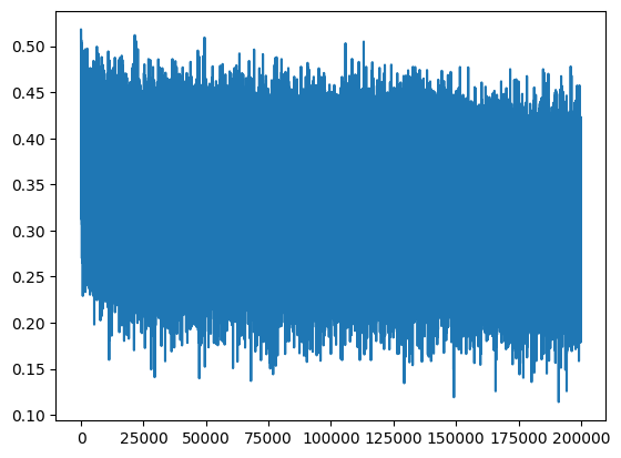
The plot for lossi looks very crazy, it’s because the batch size of 32 is way too few so this time we got lucky, and next time we got unlucky. And the mini-batch loss splashed too much. We should probably fix it.

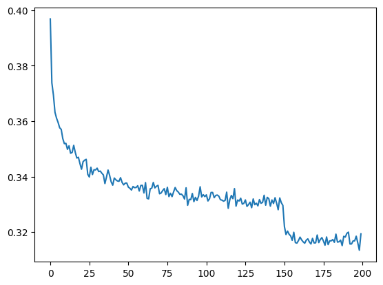
We pivot to a row for every 1000 observations of lossi and calculate the mean, we end up have 200 observations which is easier to see.

plt.plot(torch.tensor(lossi).view(-1, 1000).mean(1))

We can also observe the learning rate decay at 150k training loops.

lossi plot fixed

pytorchifying our code: layers, containers, torch.nn, fun bugs

Now we notice that we still have the embedding operation lying outside the pytorch-ified layers. It basically creating a lookup table C, embedding it with our data Y (or Yb), then stretching out to row with view() which is very cheap in PyTorch as no more memory creation is needed.

We modulize this by constructing 2 classes:

class Embedding:
  
  def __init__(self, num_embeddings, embedding_dim):
    self.weight = torch.randn((num_embeddings, embedding_dim))
    
  def __call__(self, IX):
    self.out = self.weight[IX]
    return self.out
  
  def parameters(self):
    return [self.weight]

# -----------------------------------------------------------------------------------------------
class Flatten:

  def __call__(self, x):
    self.out = x.view(x.shape[0], -1)
    return self.out
  
  def parameters(self):
    return []

Now we can re-define the layers like this:

layers = [
  Embedding(vocab_size, n_embd),
  Flatten(),
  Linear(n_embd * block_size, n_hidden, bias=False),
  BatchNorm1d(n_hidden),
  Tanh(),
  Linear(n_hidden, vocab_size),
]

and also remove the C, emb definition in the forward pass construction. Going futher, we will be not only pytorchifying the elements of layers only, but also the layers itself. In PyTorch, we have term containers, which specifying how we organize the layers in a network. And what are we doing here is constructing layers sequentially, which is equivalent to Sequential in the containers:

class Sequential:
  
  def __init__(self, layers):
    self.layers = layers
  
  def __call__(self, x):
    for layer in self.layers:
      x = layer(x)
    self.out = x
    return self.out
  
  def parameters(self):
    # get parameters of all layers and stretch them out into one list
    return [p for layer in self.layers for p in layer.parameters()]

and wrapp the layers into our model:

model = Sequential([
  Embedding(vocab_size, n_embd),
  Flatten(),
  Linear(n_embd * block_size, n_hidden, bias=False),
  BatchNorm1d(n_hidden),
  Tanh(),
  Linear(n_hidden, vocab_size),
])

2 implementing WaveNet

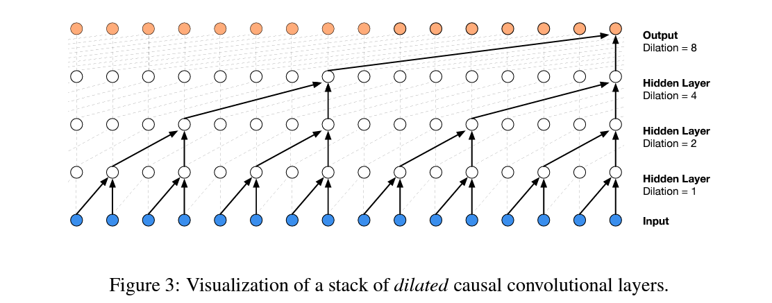
So far with the classical MLP following Bengio et al. (2003), we have a embedding layer followed by a hidden layer and end up with a activation layer. Although we added more layer after the embedding, we could not make a significant progress.

The problem is we dont have a naive way of making the model bigger in a productive way. We are still in the case that we crushing all the characters into a single all the way at the begining. And even if we make this a bigger layer and add neurons it’s still like silly to squash all that information so fast into a single step.

overview: WaveNet

Visualization of the WaveNet idea - Progressive Fusion

dataset bump the context size to 8

first we change the block_size into 8 and now our dataset looks like:

........ ---> y
.......y ---> u
......yu ---> h
.....yuh ---> e
....yuhe ---> n
...yuhen ---> g
..yuheng ---> .
........ ---> d
.......d ---> i
......di ---> o
.....dio ---> n
....dion ---> d
...diond ---> r
..diondr ---> e
.diondre ---> .
........ ---> x
.......x ---> a
......xa ---> v
.....xav ---> i
....xavi ---> e

The model size now bumps up to 22k.

re-running baseline code on block_size = 8

Just by lazily extending the context size to 8, we can already improve the model a little bit, the loss on validation split now is around 2.045. The names generated now look prettier:

zamari.
brennis.
shavia.
wililke.
obalyid.
leenoluja.
rianny.
jordanoe.
yuvalfue.
ozleega.
jemirene.
polton.
jawi.
meyah.
gekiniq.
angelinne.
tayler.
catrician.
kyearie.
anderias.

Let’s deem this as a baseline then we can start to implement WaveNet and see how far we can go!

implementing WaveNet

First, let’s revisit the shape of the tensors along the way of the forward pass in our neural net:

# Look at a batch of just 4 examples
ix = torch.randint(0, Xtr.shape[0], (4,))
Xb, Yb = Xtr[ix], Ytr[ix]
logits = model(Xb)
print(Xb.shape)
Xb

# > torch.Size([4, 8]) # because the context length is now 8
# > tensor([[ 0,  0,  0,  0,  0,  0, 13,  9],
#         [ 0,  0,  0,  0,  0,  0,  0,  0],
#         [ 0,  0,  0, 11,  5, 18, 15, 12],
#         [ 0,  0,  4, 15, 13,  9, 14,  9]])

# Output of the embedding layer, each input is translated
# to 10 dimensional vector
model.layers[0].out.shape
# > torch.Size([4, 8, 10])

# Output of Flatten layer, each 10-dim vector is concatenated
# to each other for all 8-dim context vectors
model.layers[1].out.shape
# > torch.Size([4, 80])

# Output of the Linear layer, take 80 and create 200 channels,
# just via matrix mult
model.layers[2].out.shape
# > torch.Size([4, 200])

Now look into the Linear layer, which take the input x in the forward pass, multiply by weight and add the bias in (there is broadcasting here). So the transformation in this layer looks like:

(torch.randn(4, 80) @ torch.randn(80, 200) + torch.randn(200)).shape

# > torch.Size([4, 200])

Input x matrix here does not need to be 2 dimensional array. The matrix multiplication in PyTorch is quite powerfull, you can pass more than 2 dimensional array. And all dimensions will be preserved except the last one. Like this:

(torch.randn(4, 5, 80) @ torch.randn(80, 200) + torch.randn(200)).shape

# > torch.Size([4, 5, 200])

Which we want to improve now is not just flatten the 8 characters input too fast at the beginning, we want to group them pair by pair to process them in parallel.

(x1 x2) (x3 x4) (x5 x6) (x7 x8)

Particularly for 8 characters block size we want to divide it into 4 groups ~ 4 pair of bigrams. We are increasing the dimensions of the batch.

(torch.randn(4, 4, 20) @ torch.randn(20, 200) + torch.randn(200)).shape

# > torch.Size([4, 4, 200])

How can we achieve this in PyTorch, we can index the odd and even indexes then pair them up.

e = torch.randn(4, 8, 10) # 4 examples, 8 chars context size, 10-d embedding
# goal: want this to be (4, 4, 20) where consecutive 10-d vectors get concatenated

explicit = torch.cat([e[:, ::2, :], e[:, 1::2, :]], dim=2) # cat in the third dim
explicit.shape 
# > torch.Size([4, 4, 20])

Of course, PyTorch provide a more efficient way to do this, using view():

(e.view(4, 4, 20) == explicit).all()
# > tensor(True)

We are going to modulize the FlattenConsecutive:

class FlattenConsecutive:
  
  def __init__(self, n):
    self.n = n
    
  def __call__(self, x):
    B, T, C = x.shape
    x = x.view(B, T//self.n, C*self.n)
    if x.shape[1] == 1: # spurious tensor, if it's 1, squeeze it
      x = x.squeeze(1)
    self.out = x
    return self.out
  
  def parameters(self):
    return []

and update the flatten layer to FlattenConsecutive(block_size) (8) in our model. We can observe the dimension of tensors in all layers:

for layer in model.layers:
  print(layer.__class__.__name__,": ", tuple(layer.out.shape))

# Embedding :  (4, 8, 10)
# Flatten :  (4, 80)
# Linear :  (4, 200)
# BatchNorm1d :  (4, 200)
# Tanh :  (4, 200)
# Linear :  (4, 27)

This is what we have currently. But as said, we dont want to flatten too fast, so we gonna flatten by 2 character, here is the update of the model - 3 layers present the consecutive flatten 4 -> 2 -> 1:

model = Sequential([
  Embedding(vocab_size, n_embd),
  FlattenConsecutive(2), Linear(n_embd * 2, n_hidden, bias=False), BatchNorm1d(n_hidden), Tanh(),
  FlattenConsecutive(2), Linear(n_hidden*2, n_hidden, bias=False), BatchNorm1d(n_hidden), Tanh(),
  FlattenConsecutive(2), Linear(n_hidden*2, n_hidden, bias=False), BatchNorm1d(n_hidden), Tanh(),
  Linear(n_hidden, vocab_size),
])

and here is tensors dimension flowing in forward pass:

Embedding :  (4, 8, 10)
FlattenConsecutive :  (4, 4, 20)
Linear :  (4, 4, 200)
BatchNorm1d :  (4, 4, 200)
Tanh :  (4, 4, 200)
FlattenConsecutive :  (4, 2, 400)
Linear :  (4, 2, 200)
BatchNorm1d :  (4, 2, 200)
Tanh :  (4, 2, 200)
FlattenConsecutive :  (4, 400)
Linear :  (4, 200)
BatchNorm1d :  (4, 200)
Tanh :  (4, 200)
Linear :  (4, 27)

That’s is, we have successfully implemented the WaveNet.

training the WaveNet: first pass

Now assume we use the same size of network (number of neurons), let’s see if the loss can be improved. We change the n_hidden = 68, so that the total parameters of our network remain 22k. Below is update tensor dims for a batch (32):

Embedding :  (32, 8, 10)
FlattenConsecutive :  (32, 4, 20)
Linear :  (32, 4, 68)
BatchNorm1d :  (32, 4, 68)
Tanh :  (32, 4, 68)
FlattenConsecutive :  (32, 2, 136)
Linear :  (32, 2, 68)
BatchNorm1d :  (32, 2, 68)
Tanh :  (32, 2, 68)
FlattenConsecutive :  (32, 136)
Linear :  (32, 68)
BatchNorm1d :  (32, 68)
Tanh :  (32, 68)
Linear :  (32, 27)

It turns out that we got almost identical result. There are 2 things:

1. We just constructed the architecture of WaveNet but not tortured the model enough to find best set of hyperparameters; and
2. We may have a bug in BatchNorm1d layer, let’s take a look into this.

fixing batchnorm1d bug

Let’s look at the BatchNorm1d happen in the first flatten layer:

e = torch.randn(32, 4 , 68)
emean = e.mean(0, keepdim = True) # 1, 4, 68
evar = e.var(0, keepdim = True) # 1, 4, 68

ehat = (e - emean) / torch.sqrt(evar + 1e-5)
ehat.shape

# > torch.Size([32, 4, 68])

For ehat, everything is calculated properly, mean and variance are calculated to the batch and the 2nd dim 4 is preserved. But for the running_mean:

model.layers[3].running_mean.shape

# > torch.Size([1, 4, 68])

We see it is (1, 4, 68) while we are expected it’s 1 dimensional only which is defined in the init method (torch.zeros(dim)). We are maintaining the batch norm in parallel over 4 x 68 channels individually and independently instead of just 68 channels. We want to treat this 4 just like a batch norm dimension, ie everaging of 32 * 4 numbers for 68 channels. Fortunately PyTorch mean() method offer the reducing dimension not only for integer but also tuple.

e = torch.randn(32, 4 , 68)
emean = e.mean((0,1), keepdim = True) # 1, 1, 68
evar = e.var((0,1), keepdim = True) # 1, 1, 68

ehat = (e - emean) / torch.sqrt(evar + 1e-5)
ehat.shape

# > torch.Size([32, 4, 68])

model.layers[3].running_mean.shape

# > torch.Size([1, 1, 68])

We now modify the BatchNorm1d definition accordingly, only the training mean/var in the __call__ method:

# ---- remains the same
  def __call__(self, x):
    # calculate the forward pass
    if self.training:
      if x.ndim == 2:
        dim = 0
      elif x.ndim == 3:
        dim = (0,1)
      xmean = x.mean(dim, keepdim=True) # batch mean
      xvar = x.var(dim, keepdim=True) # batch variance
    else:
      xmean = self.running_mean
      xvar = self.running_var
    xhat = (x - xmean) / torch.sqrt(xvar + self.eps) # normalize to unit variance
    self.out = self.gamma * xhat + self.beta
# ---- remaind the same

re-training WaveNet with bug fix

Now retraining the network with bug fixed, we obtain a slightly better loss of 2.022. We just fixed the normalization term inside the network so they did not thrush too much so a little improvement only is expected.

scaling up our WaveNet

Now we’re ready to scale up our network and retrain everything, the model now have roughly 76k paramters. We finally passed the 2.0 threshold and achieved the loss of 1.99 on the validation split.

n_embd = 24
n_hidden = 128

And here is final loss plot:

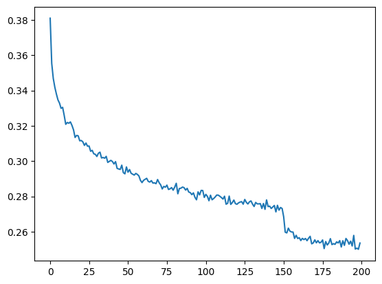
lossi final

3 conclusions

performance log

Loss logs

Step	What we did	Loss we got (accum)
1	original (3 character context + 200 hidden neurons, 12K params)	train 2.0467958450317383 val 2.0989298820495605
2	context: 3 -> 8 (22K params)	train 1.9028635025024414 val 2.044949769973755
3	flat -> hierarchical (22K params)	train 1.9366059303283691 val 2.017268419265747
4	fix bug in batchnorm1d	train 1.9156142473220825 val 2.0228867530822754
5	scale up the network: n_embd 24, n_hidden 128 (76K params)	train 1.7680459022521973 val 1.994154691696167

experimental harness

The “harness” metaphor is apt because it’s like a structured support system that allows researchers to systematically explore and optimize neural network configurations, much like a harness helps guide and support an athlete during training.

Note

An experimental harness typically includes several key components:

1. Hyperparameter Search Space Definition: This involves specifying the range of hyperparameters to be explored, such as:

• Learning rates
• Batch sizes
• Network architecture depths
• Activation functions
• Regularization techniques
• Dropout rates

2. Search Strategy: Methods for exploring the hyperparameter space, which can include:

• Grid search
• Random search
• Bayesian optimization
• Evolutionary algorithms
• Gradient-based optimization techniques

3. Evaluation Metrics: Predefined metrics to assess model performance, such as:

• Validation accuracy
• Loss function values
• Precision and recall
• F1 score
• Computational efficiency

4. Automated Experiment Management: Tools and scripts that can:

• Automatically generate and run different model configurations
• Log results
• Track experiments
• Compare performance across different hyperparameter settings

5. Reproducibility Mechanisms: Ensuring that experiments can be repeated and validated, which includes:

• Fixed random seeds
• Consistent data splitting
• Versioning of datasets and configurations

WaveNet but with “dilated causal convolutions”

• Convolution is a “for loop” applying a linear filter over space of some input sequence;
• Not happen only in Python but also in Kernel

torch.nn

We have implement alot of concepts in torch.nn:

• containers: Sequential
• Linear, BatchNorm1d, Tanh, FlattenConsecutive, …

the development process of building deep neural nets & going forward

• Spending a ton of time exploring PyTorch documentation, unfortunately it’s not a good one;
• Ton of time to make the shapes work: fan in, fan out, NLC or NLC, broadcasting, viewing, etc;
• What we:
  • done: implemented dilated causal convoluntional network;
  • to be explores: residual and skip connections;
  • to be explores: experimental harness;
  • more mordern networks: RNN, LSTM, Transformer.

4 resources

1. WaveNet 2016 from DeepMind: https://arxiv.org/abs/1609.03499;
2. Bengio et al. 2003 MLP LM: https://www.jmlr.org/papers/volume3/bengio03a/bengio03a.pdf;
3. Notebook: https://github.com/karpathy/nn-zero-to-hero/blob/master/lectures/makemore/makemore_part5_cnn1.ipynb;
4. DeepMind’s blog post from 2016: https://deepmind.google/discover/blog/wavenet-a-generative-model-for-raw-audio/